Vector Embeddings & Similarity: The Foundation of RAG
Note: This post was AI-generated from rough notes using the blog generation workflow.
If you’ve worked with RAG (Retrieval-Augmented Generation) systems, you’ve probably heard the phrase “vector embeddings” thrown around a lot. But what actually are they, and why does the math underneath matter? This post breaks it down — from what an embedding is, to why cosine similarity is the right tool for comparing them, to how all of this plugs into real retrieval pipelines.
What Is a Vector Embedding?
A vector embedding is just a list of numbers. That’s it. But what those numbers represent is the interesting part — they encode the semantic meaning of a piece of text, not the words themselves.
When you feed “I love dogs” into an embedding model, you don’t get back a bag of words or a frequency count. You get back something like [0.23, -0.87, 0.41, ..., 0.06] — a list of 768 to 1536 floating point numbers that captures the concept behind the phrase.
The magic: texts with similar meanings produce vectors that point in similar directions in that high-dimensional space. The model has learned, from enormous amounts of text, that “dog” and “canine” are related, that “adore” and “love” are nearly synonymous, and that none of those words have much to do with stock markets.
Seeing It In Numbers
Let me make this concrete. Using sentence-transformers with the all-MiniLM-L6-v2 model:
| Pair | Cosine Similarity |
|---|---|
| “I love dogs” vs “I love dogs” | 1.0000 |
| “I love dogs” vs “I adore puppies” | 0.6831 |
| “I love dogs” vs “Stock markets fell” | 0.0197 |
These numbers match your intuition perfectly. Identical sentences score 1.0. Two sentences with different words but the same meaning score 0.68. Two completely unrelated sentences score nearly 0.
This is the core bet that RAG systems make: if the embedding model is good, similarity scores reflect real meaning relationships.
Why Direction Matters More Than Magnitude
Here’s the insight that makes cosine similarity the right choice: in embedding space, direction encodes meaning, not magnitude.
Imagine two descriptions of the same product — one terse (“Fast, reliable SSD”), one verbose (“This is an extremely fast and highly reliable solid-state drive with excellent performance characteristics”). The verbose one produces a longer vector. The terse one produces a shorter vector. But both vectors point in the same direction.
If you just subtracted the vectors or measured straight-line distance, the different magnitudes would throw off your comparison. A short document and a long document about the same topic would look more different than they actually are.

Cosine similarity solves this by measuring the angle between two vectors, completely ignoring how long they are. Two vectors pointing in exactly the same direction have a 0° angle — cosine similarity of 1.0. Perpendicular vectors (90°) score 0.0. Opposite vectors (180°) score -1.0.
The Math: Cosine Similarity
The formula is straightforward:
cos(θ) = (A · B) / (|A| × |B|)
A · Bis the dot product — multiply corresponding elements and sum them up|A|and|B|are the magnitudes of each vector — square root of the sum of squares- Dividing by the magnitudes normalizes out the scale, leaving only the directional relationship
In Python, this is a few lines:
import numpy as np

def cosine_similarity(a, b):
    dot_product = np.dot(a, b)
    magnitude = np.linalg.norm(a) * np.linalg.norm(b)
    return dot_product / magnitude
Or with sentence-transformers, you can skip the manual math entirely:
from sentence_transformers import SentenceTransformer, util

model = SentenceTransformer('all-MiniLM-L6-v2')

sentences = [
    "I love dogs",
    "I adore puppies",
    "Stock markets fell today"
]

embeddings = model.encode(sentences)

score = util.cos_sim(embeddings[0], embeddings[1])
print(f"'I love dogs' vs 'I adore puppies': {score.item():.4f}")
# Output: 0.6831
You can find a complete runnable version in the repo: 01_cosine_similarity.py
Why Not Just Use Euclidean Distance?
Fair question. Euclidean distance measures the straight-line distance between two points in space — it’s intuitive and works fine in some cases. But it’s sensitive to magnitude, which bites you when comparing texts of different lengths.
There are three common distance metrics you’ll encounter in retrieval systems:
- Cosine similarity — measures the angle between vectors; scale-invariant; best for semantic text comparison
- Euclidean distance — measures straight-line distance; magnitude-sensitive; works well when vectors are normalized to unit length
- Dot product — combines angle and magnitude; used in some retrieval systems where longer, more detailed documents should naturally score higher
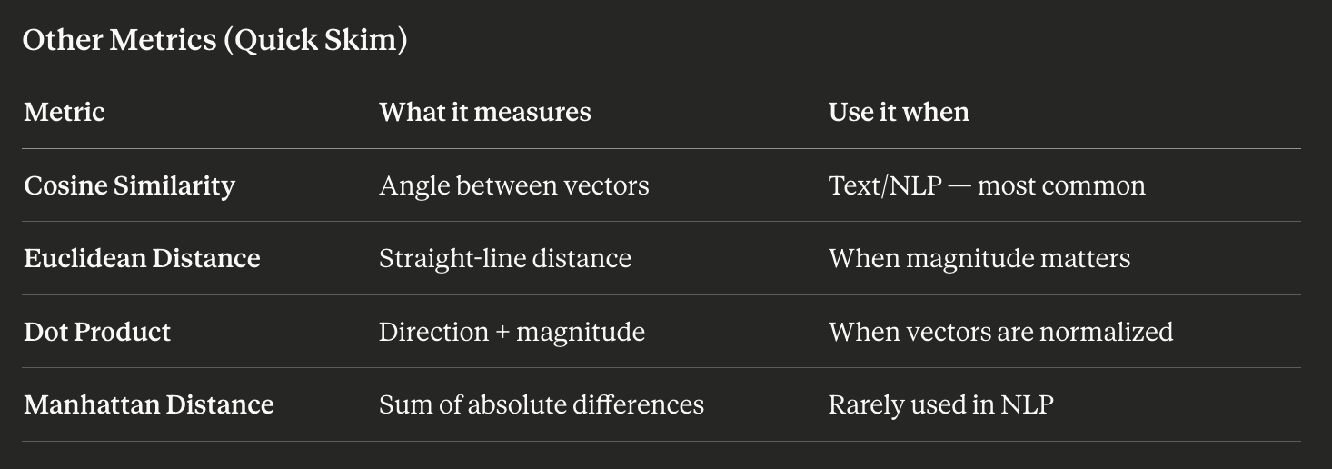
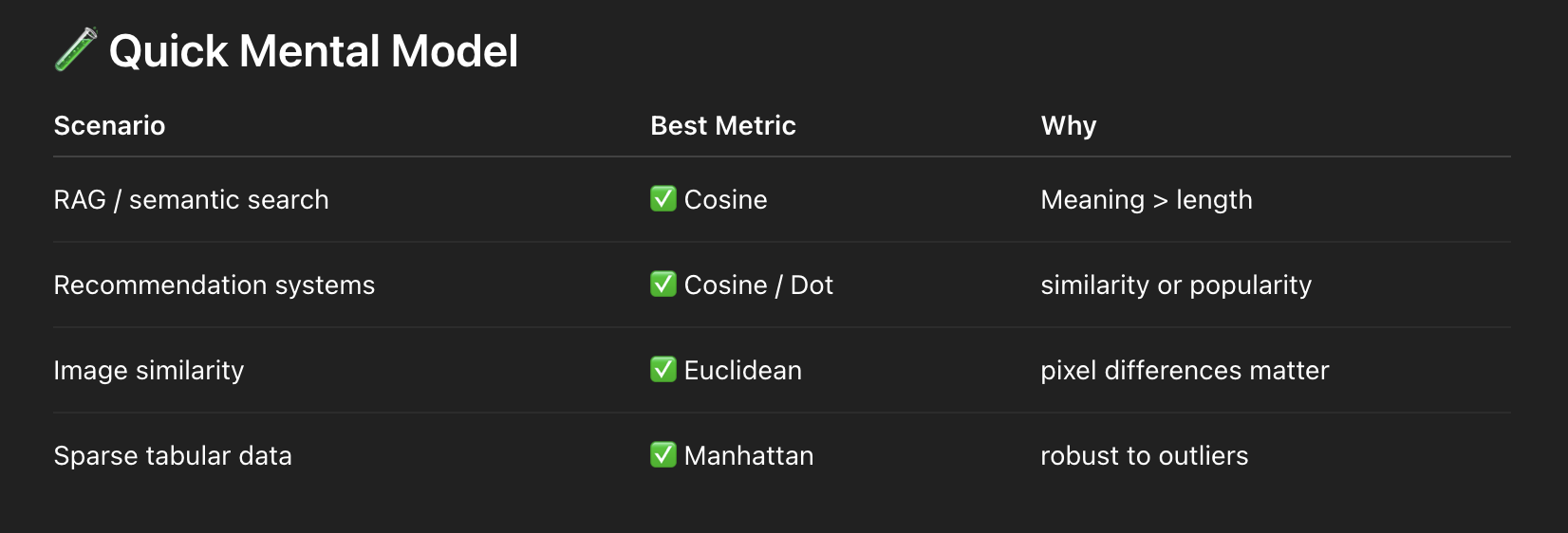
For most RAG use cases, cosine similarity is the right default. It’s scale-invariant, well-understood, and maps cleanly to the question you’re actually asking: how similar is the meaning of these two texts?
The demo at 02_why_cosine.py walks through a side-by-side comparison of all three metrics so you can see exactly where Euclidean distance goes wrong on unnormalized embeddings.
Step-by-Step Intuition: Zero Words in Common, High Similarity
Consider these two sentences:
- “The dog ran”
- “A canine was running”
They share zero words. A keyword search would return zero overlap. But an embedding model knows that “dog” and “canine” refer to the same animal, and that “ran” and “was running” describe the same action. These two sentences land very close together in embedding space — high cosine similarity.
This is why embeddings beat keyword search for semantic retrieval. BM25 counts words. Embeddings capture meaning.
How This Plugs Into RAG
Here’s where all of this becomes practical. In a RAG pipeline:
- At index time, you chunk your documents and embed each chunk — storing the resulting vectors in a vector database
- At query time, you embed the user’s question using the same model
- You compute cosine similarity between the query vector and every stored document vector
- You return the top-k most similar chunks as context for the LLM
def retrieve(query, document_chunks, model, top_k=3):
    query_embedding = model.encode(query)
    chunk_embeddings = model.encode(document_chunks)

    scores = util.cos_sim(query_embedding, chunk_embeddings)[0]
    top_results = scores.topk(top_k)

    return [(document_chunks[i], scores[i].item())
            for i in top_results.indices]
The retrieval step is entirely built on this similarity score. If the score is accurate, relevant context reaches the LLM. If it’s not, the LLM gets garbage — and no amount of prompt engineering or model quality fixes bad retrieval.
This is why embedding model choice matters as much as LLM choice. A weak embedding model produces retrieval that looks plausible but misses the point. The LLM then confidently answers based on the wrong context.
A Note on Embedding Models
Not all embedding models are equal. all-MiniLM-L6-v2 is fast and good for prototyping. For production, look at:
text-embedding-3-large(OpenAI) — strong general-purpose performancebge-large-en-v1.5(BAAI) — excellent open-source optionE5-mistral-7b-instruct— higher quality at higher compute cost
The MTEB leaderboard is the canonical benchmark for comparing them on retrieval tasks.
Wrapping Up
Vector embeddings convert text meaning into geometry. Cosine similarity measures how aligned that geometry is. Together, they form the retrieval layer of every RAG system worth building.
The key things to internalize:
- Embeddings capture semantics, not syntax — “dog” and “canine” end up close in embedding space
- Direction encodes meaning; magnitude encodes verbosity — cosine similarity handles this correctly
- The formula is simple: dot product divided by the product of magnitudes
- Bad embeddings break RAG at the foundation — retrieval quality is a ceiling on overall system quality
If you want to play with this yourself, the full code is in the repo linked above. Running 01_cosine_similarity.py and 02_why_cosine.py back to back gives you a solid feel for how the numbers behave across different sentence pairs and distance metrics.