The Evolution: Beyond Transformers
Note: This post was AI-generated from rough notes using the blog generation workflow.
The original 2017 Transformer was built for one job: translation. You have a source sentence in French, you want it in English. The encoder reads the source, builds a rich representation, and hands it off to the decoder via cross-attention. Clean. Logical. But also a hint redundant the moment your input and output are the same language.
From Encoder-Decoder to Decoder-Only
The key insight behind GPT and everything that followed is simple: predicting the next token doesn’t need two halves. Understanding and generation are the same operation. If you can predict what comes next given everything before, you’re doing both simultaneously.
Going decoder-only required exactly three concrete changes:
- Cross-attention removed entirely. No encoder means no cross-attention sub-layer. Each block keeps self-attention and FFN, nothing else.
- Causal masking everywhere. Instead of a padding mask, every token only attends to itself and what came before. The future is invisible.
- Prompt and response are one stream. There’s no encoder input vs. decoder input distinction. Your question and the model’s answer are just tokens, concatenated.
# Causal mask — token i cannot see token j if j > i
def causal_mask(seq_len):
    mask = torch.tril(torch.ones(seq_len, seq_len))
    return mask.masked_fill(mask == 0, float('-inf'))
The payoff is significant. All parameters serve one job. The model scales better with depth because every layer is doing the same thing — predicting forward. And every task (translation, coding, QA, summarization, chat) collapses into the same problem: predict the next token. That uniformity is why GPT-style models generalize the way they do.
The Three Variants in the Wild
It’s worth keeping the three main Transformer families straight:
| Architecture | Examples | Sweet Spot |
|---|---|---|
| Encoder-only | BERT, RoBERTa | Classification, search, embeddings |
| Encoder-decoder | T5, BART | Translation, summarization |
| Decoder-only | GPT, Claude, Gemini | General generation |
Encoder-only models are still the right tool for embedding text or running classifiers. Encoder-decoder models still show up in specialized translation pipelines. But when people say “LLM” today, they mean decoder-only.
The Attention Bottleneck
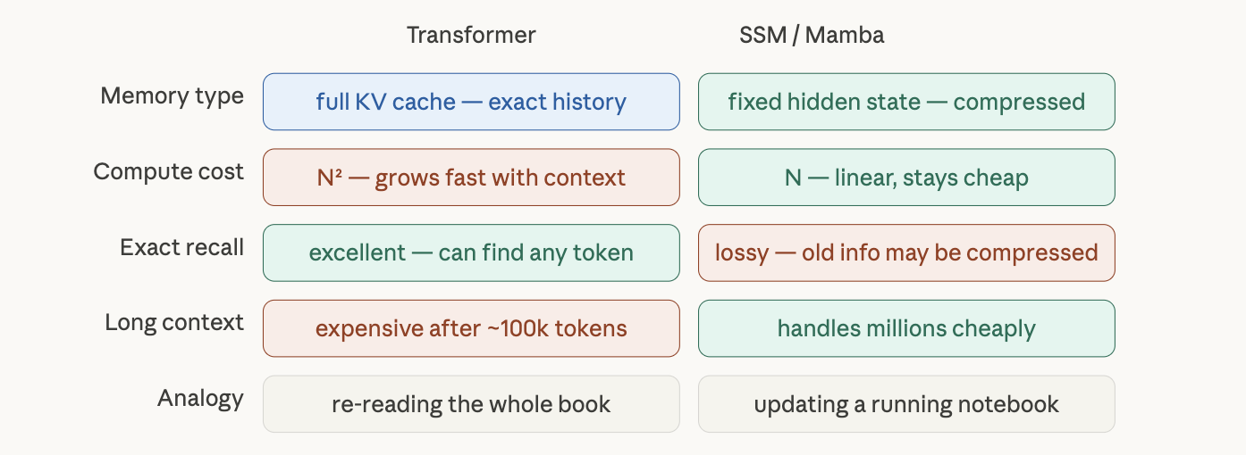
Decoder-only scaling hit a hard wall: attention is O(N²). Every token attends to every other token. Double the sequence length, quadruple the compute. At 1M tokens, this isn’t slow — it’s a wall.
The KV cache compounds it. During inference, each generated token’s Keys and Values get stored in GPU memory so you don’t recompute them. Long conversations exhaust memory fast. Running long-context serving at scale gets expensive quickly.
This is the problem that opened the door for a different approach entirely.
State Space Models: A Different Mental Model
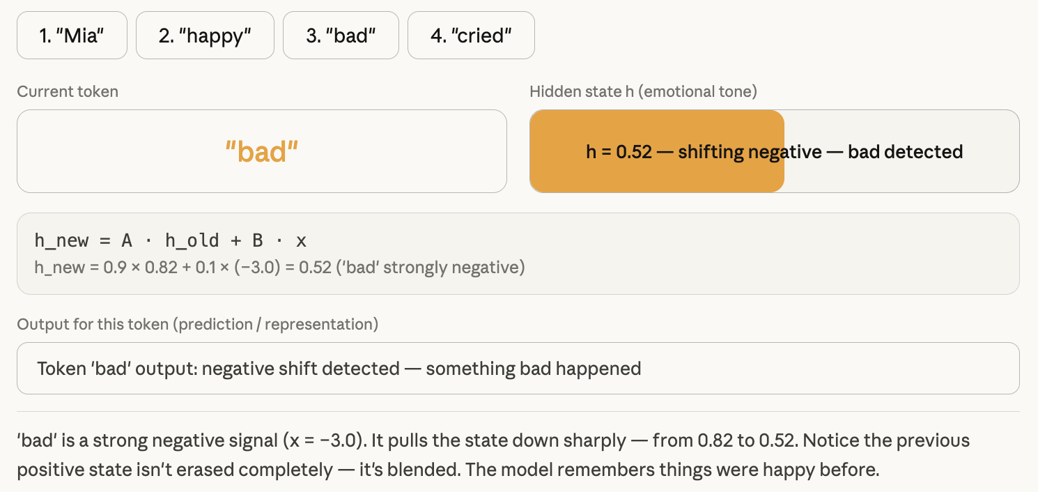
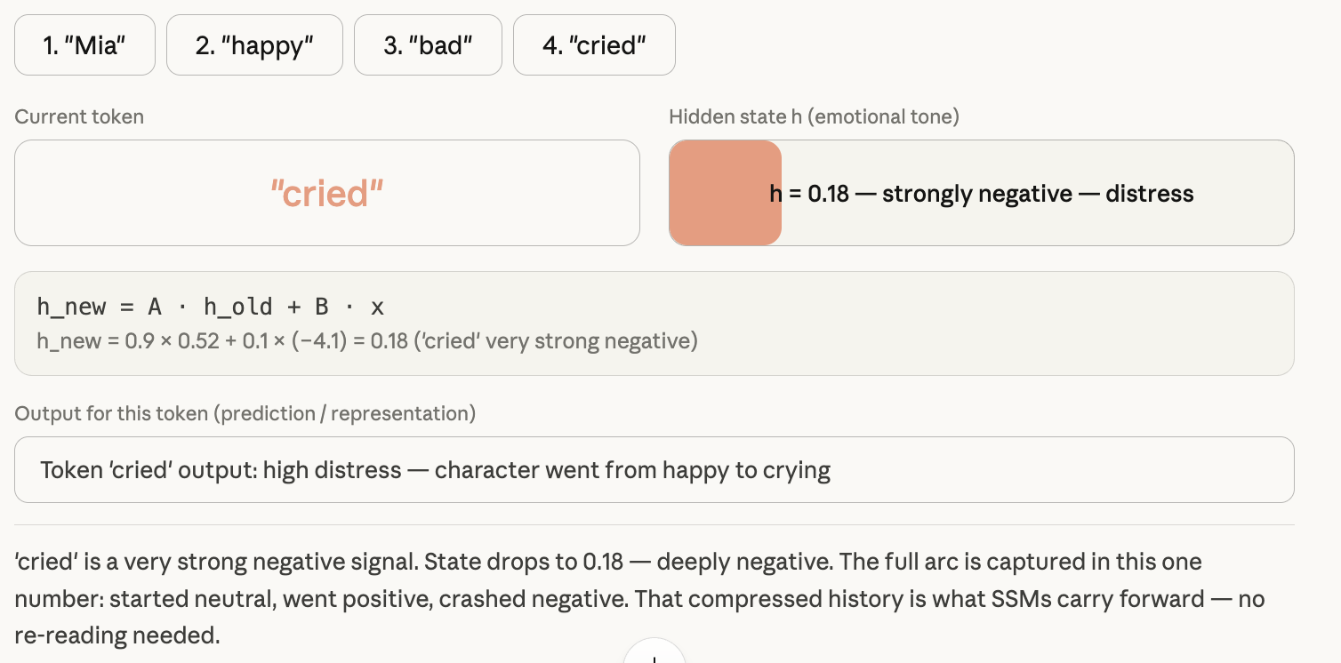
SSMs come from control theory — the math behind autopilots and cruise control. Instead of attending to everything, the model maintains a single compressed hidden state updated with each new token. Think of it as updating a running notebook rather than re-reading the whole book every time.
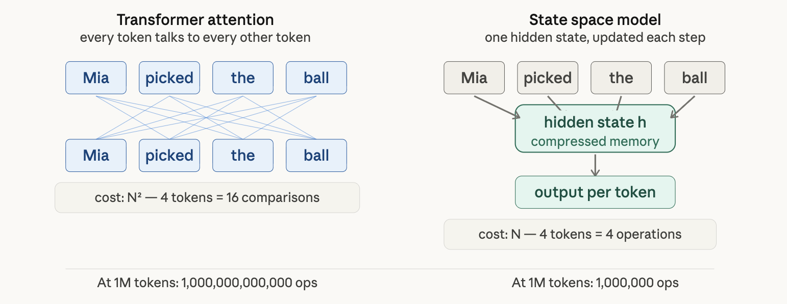
The core SSM formula is three lines:
h_new = A·h_old + B·x   # update the hidden state
y     = C·h             # read the output from state
- A = memory retention rate (how much of the past to keep)
- B = how much of the new input to absorb
- C = how to read the state to produce output
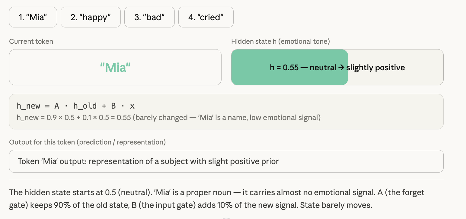
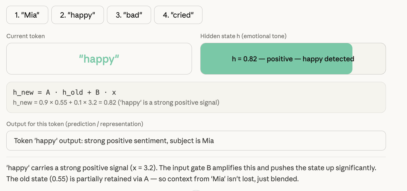
This runs in O(N) time and O(1) memory per step. The scaling math is completely different from attention.
The Fatal Flaw of Early SSMs
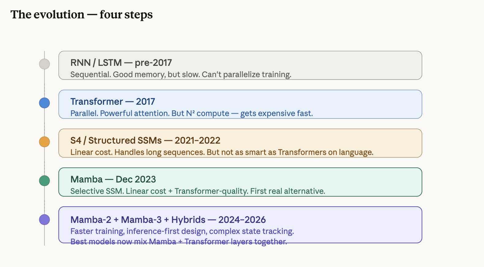
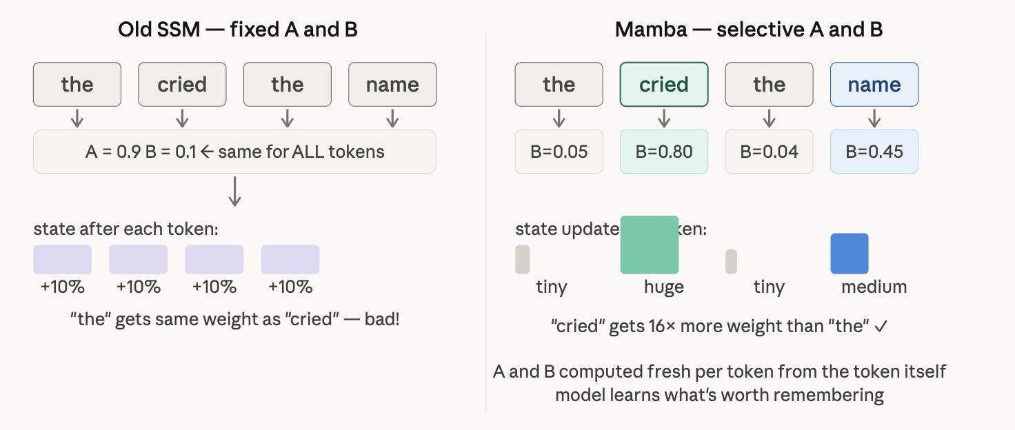
S4 (2022) showed SSMs could work for long sequences. But it had a critical problem: A and B were fixed constants. The model forgot at the same rate no matter what it was reading. “The” and “cried” were processed identically. No selectivity.
A model that can’t decide what to remember isn’t useful for language. You need to absorb emotionally significant tokens and skim filler words. Fixed parameters can’t do that.
Mamba: Selectivity Changes Everything
Mamba (December 2023) fixed this with one structural change: A and B became functions of the current input token x.
# Fixed SSM (S4): parameters are constants
A = nn.Parameter(torch.randn(d_state, d_state))
B = nn.Parameter(torch.randn(d_state, d_input))

# Mamba: parameters are input-dependent projections
def selective_update(x, h, A_log, B_proj, C_proj):
    A = -torch.exp(A_log)          # learned, but stable
    B = B_proj(x)                  # function of current token
    C = C_proj(x)                  # function of current token
    h_new = torch.exp(A) * h + B * x
    y = (C * h_new).sum(dim=-1)
    return h_new, y
During training, the model learns to absorb tokens that matter and skim the ones that don’t. The selectivity is learned, not hand-coded.
The results were striking: 5× higher inference throughput than same-size Transformers, linear O(N) scaling in sequence length, and Mamba-3B outperforming same-size Transformers while matching Transformers twice its size on language modeling benchmarks.
Mamba-2: Fixing the Training Problem
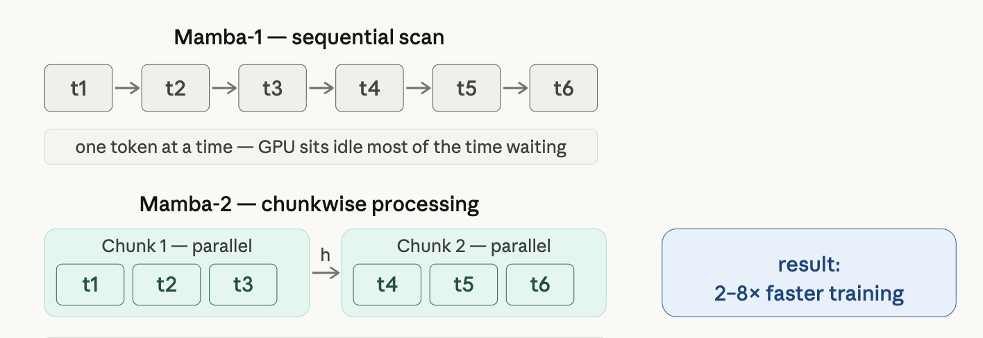
Mamba-1 had a training bottleneck. The sequential scan h_new = A·h_old + B·x requires computing tokens one-by-one — GPUs hate sequential work. They’re built for parallel matrix operations.
Mamba-2 (2024) solved this with Structured State Space Duality (SSD). The mathematical insight: SSMs and Transformers are both computing the same linear transformation through structured matrices. SSMs do it through recursive state updates; Transformers do it through direct attention. That equivalence means you can borrow Transformer GPU tricks for SSM training.
Mamba-2 introduced chunkwise processing — tokens are batched into parallel mini-batches rather than processed one-by-one. It also added Mamba heads analogous to multi-head attention, enabling tensor parallelism.
# Mamba-2 chunkwise scan (simplified)
def chunked_ssm(x, A, B, C, chunk_size=64):
    outputs = []
    h = torch.zeros(batch, d_state)
    for chunk in x.split(chunk_size, dim=1):
        # process chunk in parallel, then update state
        chunk_out, h = parallel_chunk_scan(chunk, h, A, B, C)
        outputs.append(chunk_out)
    return torch.cat(outputs, dim=1)
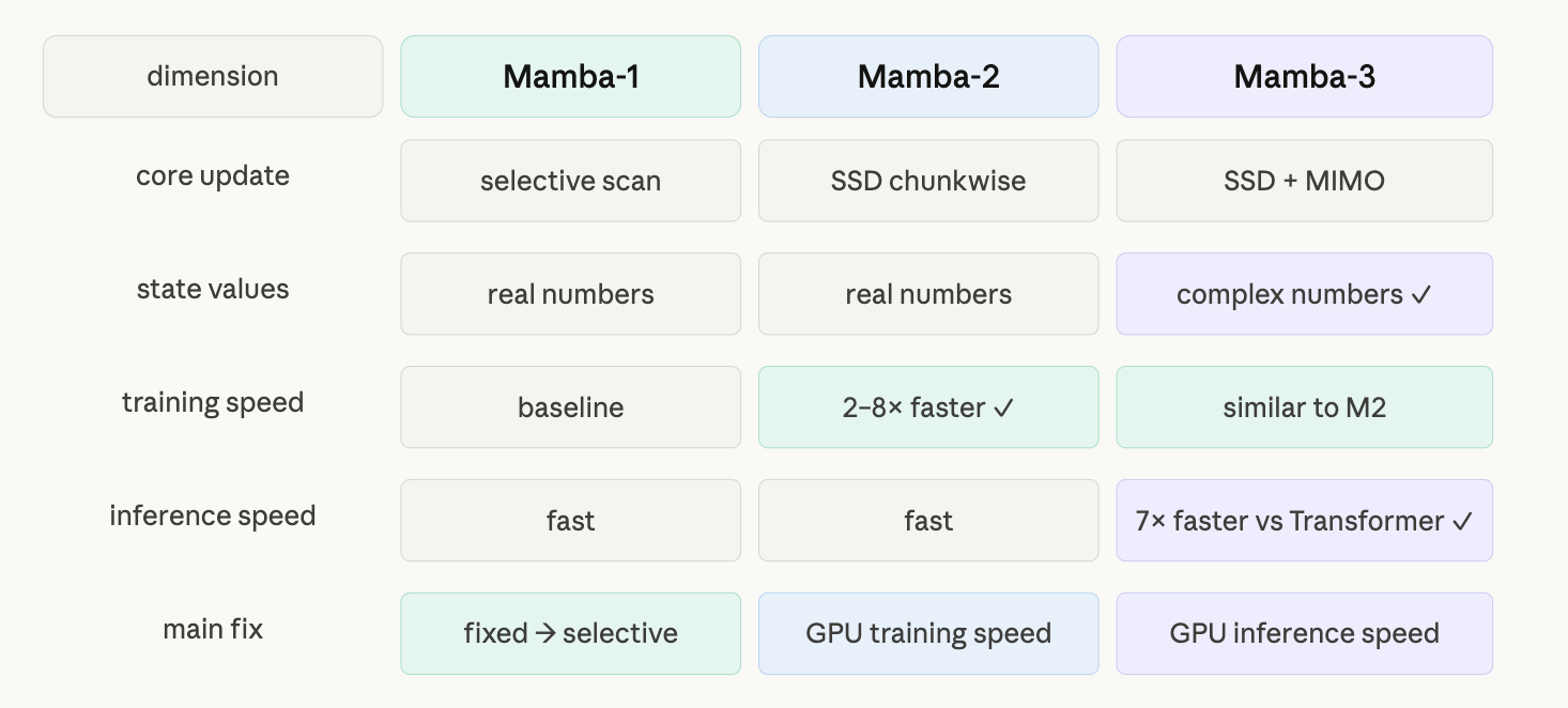
Result: 2–8× faster training while staying competitive with Transformers on language modeling benchmarks.
Mamba-3: Inference-First Design
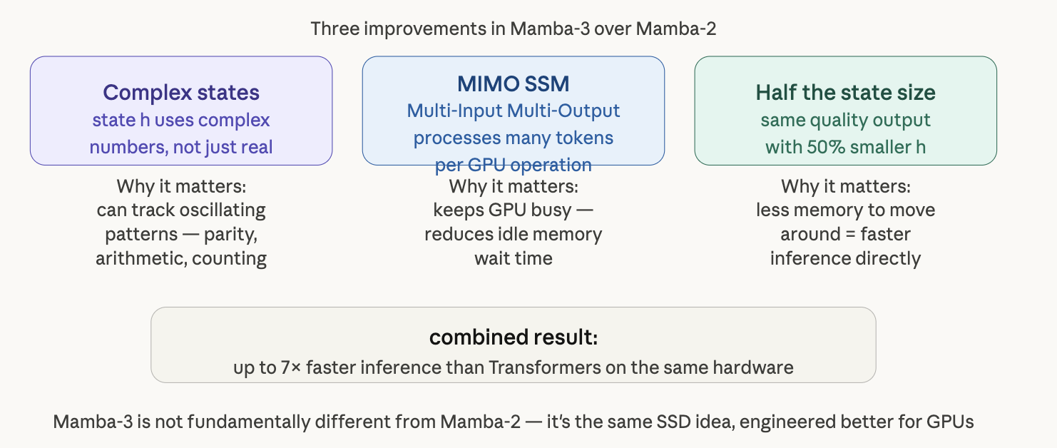
Mamba-3 (March 2026) targeted a different bottleneck: the cold GPU problem. During decoding, hardware waits on memory movement, not compute. You’re arithmetic-bound on paper but memory-bound in practice.
Mamba-3 introduced MIMO SSM (Multiple Input Multiple Output state space) — complex-valued state-space updates that boost arithmetic intensity without increasing memory footprint. This also unlocked parity and arithmetic reasoning that previous Mamba versions struggled with.
The numbers: same perplexity as Mamba-2 at half the state size, and 7× faster than Transformers on long-sequence tasks on H100 GPUs.
Hybrid Architectures: What’s Actually Winning in Production
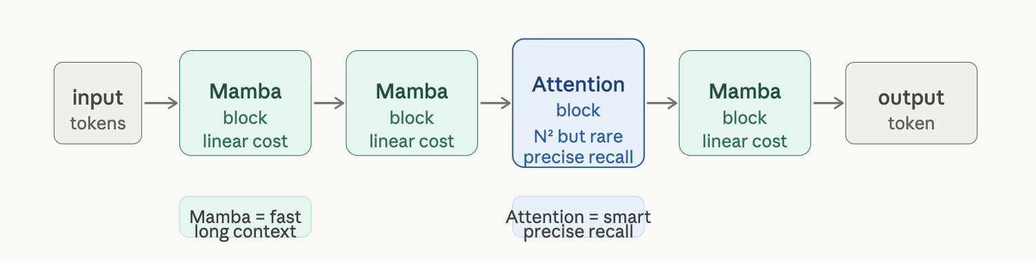
Pure Mamba has one real weakness: retrieval. A fixed-size hidden state can lose specific facts buried in long documents. If you ask “what did paragraph 47 say exactly?”, a compressed state may not have retained it.
The solution the industry landed on: interleave Mamba layers with Transformer attention layers. Mamba handles cheap long-range context. Attention handles precise retrieval. You get the best of both.
Two production examples worth knowing:
- NVIDIA Nemotron 3 Super (120B params): Mamba-Transformer hybrid with a 1M token context window
- IBM Granite 4.0: Hybrid architecture explicitly motivated by reducing serving cost
These aren’t research experiments. They’re production models built by teams that ran the cost math and made a choice.
Where This Lands
Mamba isn’t replacing Transformers. It’s being absorbed into them. The sequential scan that started in control theory for autopilots has been parallelized, scaled, and hybridized until it fits inside the same training infrastructure as attention.
The decoder-only insight — that understanding and generation are the same operation — holds. The attention bottleneck at long sequences is real. And the practical answer in 2025 is hybrid: linear scaling where you can afford approximation, precise attention where you can’t.
If you’re building systems that handle long documents, long conversations, or long code files, understanding this stack isn’t academic — it’s the difference between a system that scales and one that hits a wall at 100K tokens.