The End of the RNN Era & The Query, Key, Value Revolution
Note: This post was AI-generated from rough notes using the blog generation workflow.
If you’ve spent any time working with sequence models, you’ve probably felt the pain of RNNs before you fully understood why they hurt. Training is slow, long documents fall apart, and throwing more GPUs at the problem doesn’t help the way you’d hope. This post breaks down exactly why that is — and how the transformer’s attention mechanism fixes it at the architectural level.
The RNN Bottleneck Is Not a Hardware Problem
RNNs process tokens one at a time, left to right. Each step produces a hidden state that gets passed to the next step. That’s the design. It means token N can’t be processed until token N-1 is done, which means token N-2 has to finish before that, and so on.
This is a sequential dependency chain, and it’s baked into the architecture. You cannot parallelize it. You can buy a cluster of A100s and you’ll still be waiting for the same chain of operations to complete in order. More hardware accelerates each individual step, but it can’t run them concurrently.
That alone is a serious problem for throughput. But the deeper issue is what happens to information over distance.
What Happens to Long-Range Dependencies
Consider this sentence:
“The dog, despite the loud noise from the crowd, barked.”
For the model to correctly understand that barked is associated with dog, the signal from dog has to travel through every intermediate token before it reaches barked. The path length is O(n). Every hop through a hidden state is a compression — information gets mixed, overwritten, diluted. By the time you’re 10 or 15 tokens away, the original signal is weak.
Then vanishing gradients compound this during training. When you backpropagate through a long sequence, the gradient signal for early tokens has to travel back through all those same steps. Multiply a number slightly less than 1.0 by itself 20 times and you’re approaching zero. The model technically receives a gradient update for dog, but it’s so small that it barely moves the weights. The model learns, but poorly, from distant dependencies.
The result: RNNs work reasonably well for short sequences and fall apart for long ones. This isn’t a tuning problem. It’s a structural one.
Transformers Connect Any Two Words in O(1)
The transformer doesn’t walk the sequence. Every token connects directly to every other token in a single operation. The path length between dog and barked is 1, regardless of how many words sit between them.
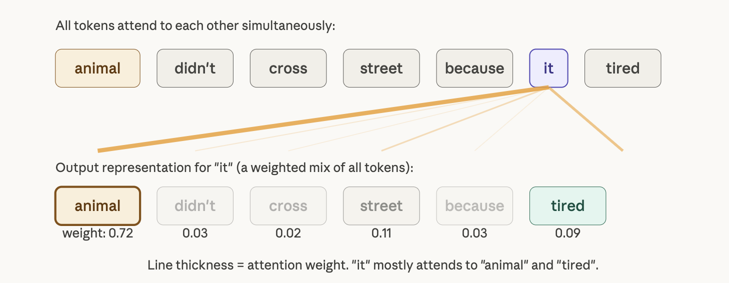
That’s the core insight. But how does the model decide which connections matter? That’s where Query, Key, and Value come in.
The Query, Key, Value Mechanism
Every token in the sequence gets assigned three vectors, learned during training:
- Query (Q): What am I looking for?
- Key (K): What do I advertise about myself?
- Value (V): What do I actually contribute if selected?
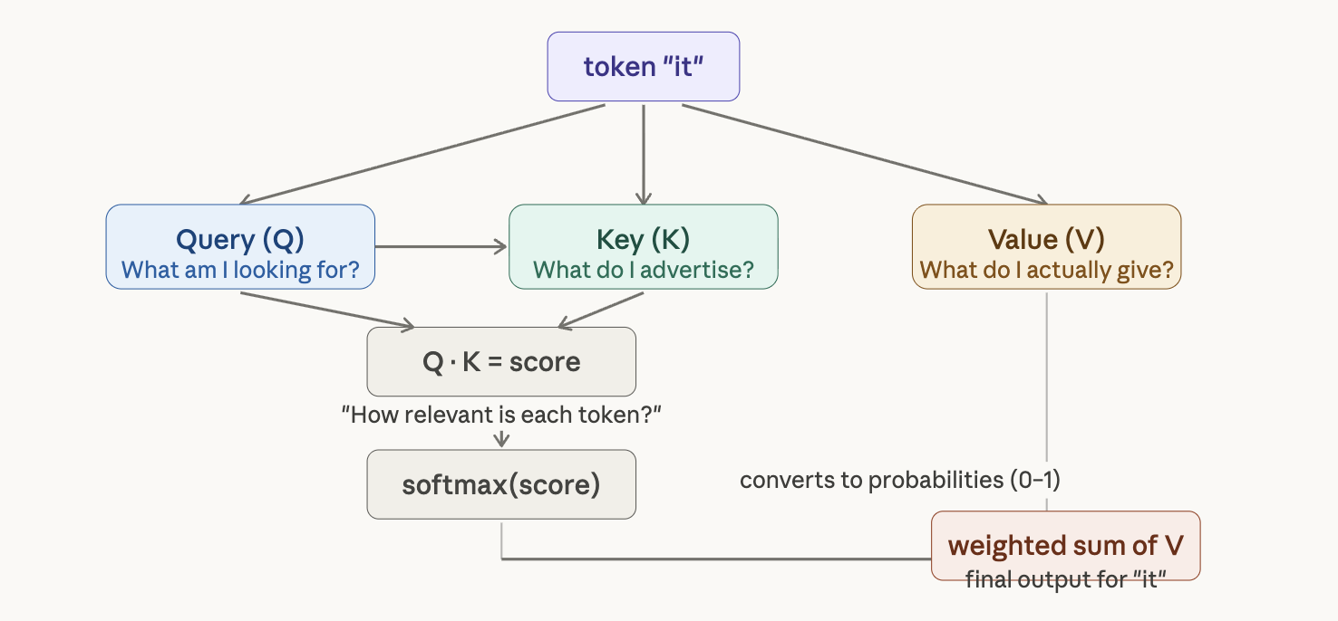
A good analogy is a library. Your search query is Q. The label on each book’s spine is K. The book’s actual content is V. The library doesn’t walk the shelves in order — it matches your query against the spine labels and hands you the relevant books directly.
Barked carries a Query vector that encodes something like “I’m a verb, I need a subject.” Dog carries a Key vector that encodes “I’m a noun, I’m a subject candidate.” The dot product between Q and K gives a compatibility score. High score = high relevance.
Step-by-Step: “The Dog Barked”
Let’s make this concrete. For the token barked, we compute its Query vector and then take the dot product with the Key vector of every token in the sentence.
import numpy as np

# Simplified example — in practice these come from learned weight matrices
Q_barked = np.array([0.8, 0.3, 0.5, 0.1])   # query for "barked"
K_the    = np.array([0.1, 0.2, 0.3, 0.4])   # key for "The"
K_dog    = np.array([0.9, 0.4, 0.6, 0.2])   # key for "dog"
K_barked = np.array([0.2, 0.1, 0.4, 0.3])   # key for "barked"

scores = {
    "The":    np.dot(Q_barked, K_the),
    "dog":    np.dot(Q_barked, K_dog),
    "barked": np.dot(Q_barked, K_barked),
}
# Raw scores → The: 1.5, dog: 4.0, barked: 0.5
Raw scores: The = 1.5, dog = 4.0, barked = 0.5. The model is already pointing at dog.
The Full Formula: Scaled Dot-Product Attention
Attention(Q, K, V) = softmax(Q · Kᵀ / √d_k) · V
Two things to unpack here: the scaling by √d_k, and the softmax.
Why Divide by √d_k?
For large embedding dimensions, dot products get large — fast. When you push large values through softmax, the output saturates. One score dominates with near-1.0 probability, everything else collapses toward 0, and the gradients in that region are effectively zero. Training stalls. This is sometimes called the “dead softmax” problem.
Dividing by √d_k keeps the scores in a reasonable range regardless of dimension size.
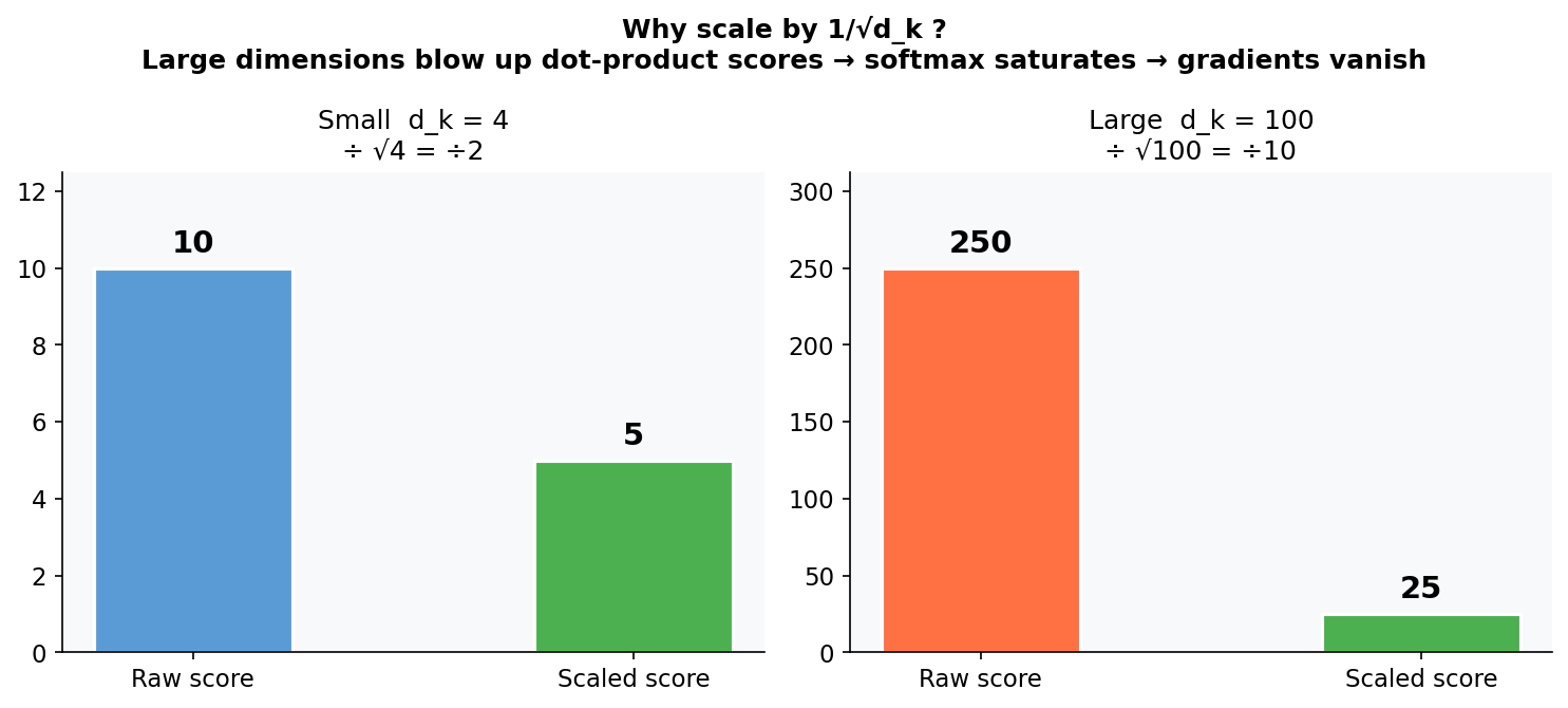
Concrete example: if d_k = 4 and your raw score is 10, scaled score is 10/2 = 5. If d_k = 100 and your raw score is 250, unscaled it causes saturation. Divide by √100 = 10 and you get 25 — manageable.
Softmax Converts Scores to Weights
After scaling, softmax normalizes the scores into a probability distribution that sums to 1.0.
def softmax(x):
    e_x = np.exp(x - np.max(x))  # subtract max for numerical stability
    return e_x / e_x.sum()

raw_scores = np.array([1.5, 4.0, 0.5])
weights = softmax(raw_scores)
# → [0.07, 0.90, 0.03]
# "The": 7%, "dog": 90%, "barked": 3%
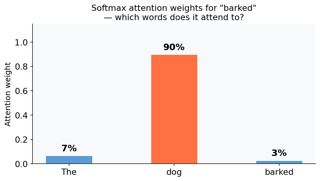
The model is now told, in a fully differentiable way: when computing the contextual representation of barked, pull 90% of your information from dog. These weights are then applied to the Value vectors to produce the final output.
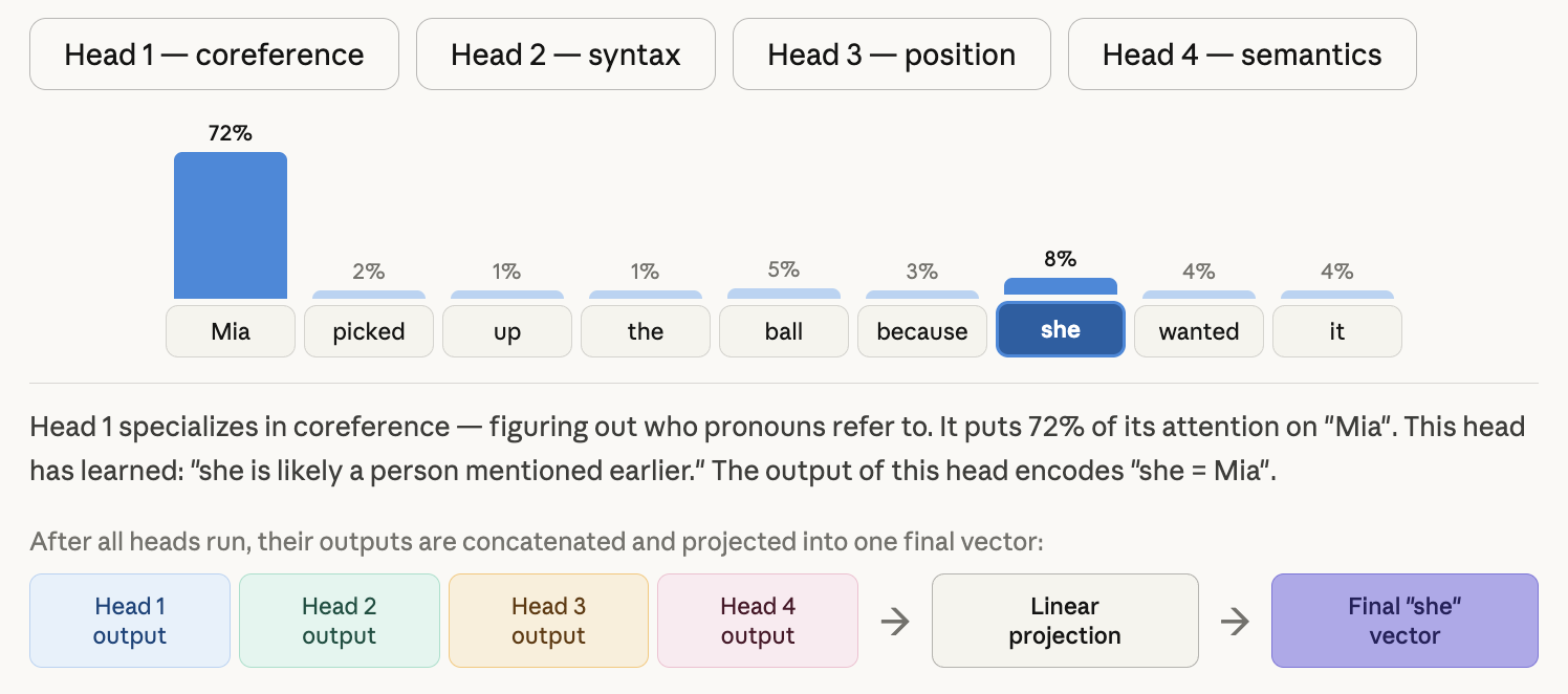
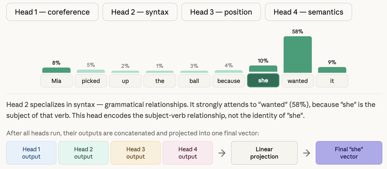
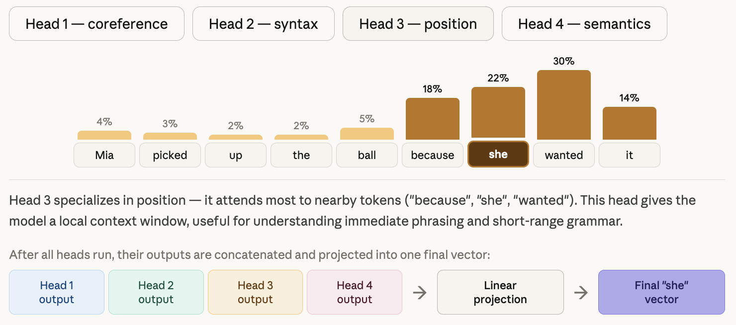
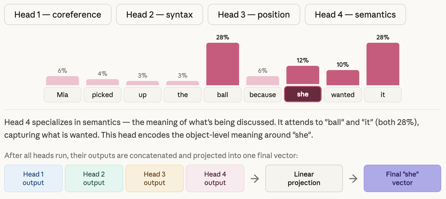
Multi-Head Attention: Running Eight Conversations in Parallel
Single-head attention produces one attention distribution per token. That means it has to compress all relationship types — syntactic subject-verb links, semantic associations, coreference, positional proximity — into one set of scores. The signal gets blurry.
Multi-head attention runs 8 (or more) independent attention heads simultaneously. Each head has its own learned weight matrices W_Q, W_K, W_V, and projects the input into a different representation subspace.
No one tells Head 1 to focus on syntax or Head 2 to focus on coreference. These roles emerge from training. Each head learns whatever pattern is most useful for the task.
After all 8 heads run in parallel, their outputs are concatenated and projected back to the model dimension through a final weight matrix W^O:
# Pseudocode — each head produces output of shape [seq_len, d_k]
head_outputs = [attention_head(Q, K, V, i) for i in range(8)]
concat = np.concatenate(head_outputs, axis=-1)  # [seq_len, 8 * d_k]
output = concat @ W_O                           # [seq_len, d_model=512]
If d_model = 512 and you have 8 heads, each head works in a 64-dimensional subspace. The concatenation reassembles a 512-dimensional output, which is projected back through W^O. All 8 heads run in parallel — no sequential dependency.
The Payoff
Pull back and look at what this architecture actually delivers:
- No sequential bottleneck. All tokens are processed in parallel. Training scales with hardware.
- O(1) path length between any two tokens. Long-range dependencies don’t degrade with distance.
- No vanishing gradient problem for long-range signals. The gradient path between dog and barked is one step, not ten.
- Multiple relationship types learned simultaneously. Multi-head attention lets the model capture syntax, semantics, and coreference in parallel without compromising any of them.
The 2017 paper “Attention Is All You Need” dropped recurrence and convolution entirely. At the time, that felt radical. Looking at the mechanics above, it makes complete sense. RNNs were doing a lot of work to compensate for their own architectural constraints. Remove the constraints, and most of that work disappears.
The transformer didn’t just improve on RNNs — it made the core problems they were struggling with structurally irrelevant.