Gradient Descent in Neural Networks: Understanding How Machines Learn
In the previous post of the neural network series, we introduced the basics of how a neural network functions, specifically with the use case of recognizing handwritten digits.
Recap: Neural Network Structure
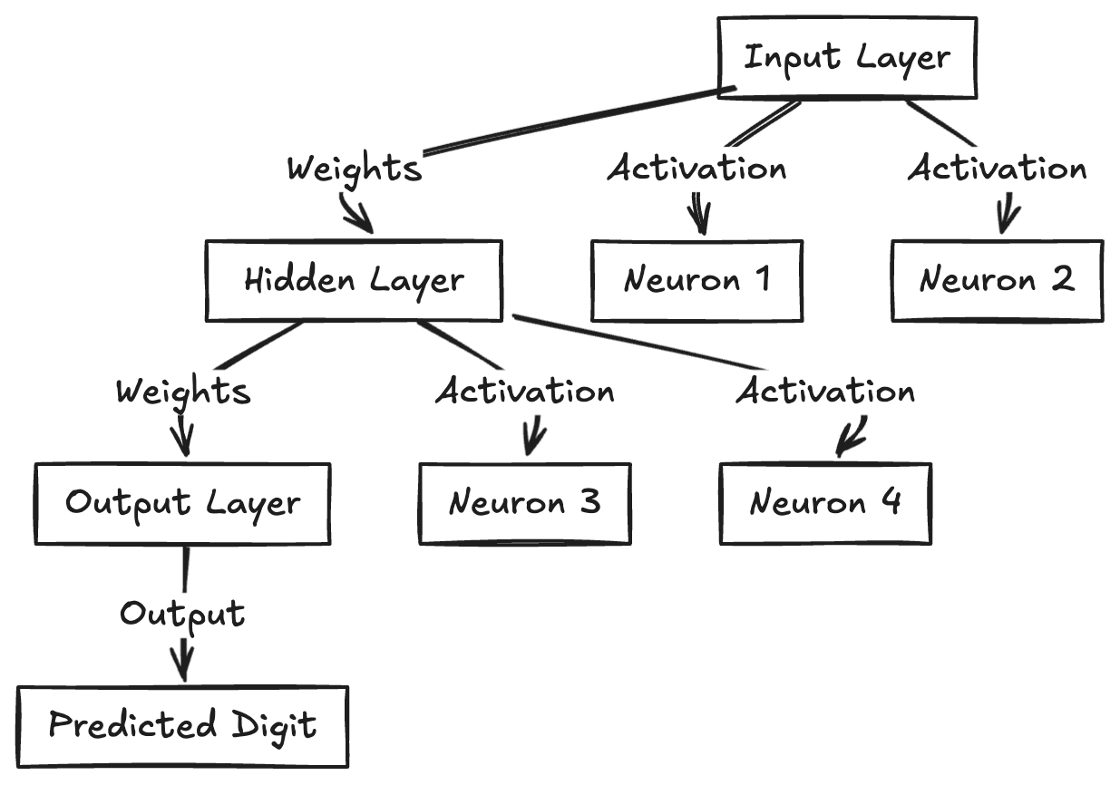
- The input layer consists of 784 neurons, each representing a pixel in a 28x28 grid of a handwritten digit.
- Each neuron’s value, called an activation, corresponds to the grayscale value of that pixel.
- The neurons are connected to each other through weights and biases—the key components that determine the network’s predictions.
- These weights and biases undergo adjustments during training to improve the network’s performance.
- The final layer consists of 10 neurons, each representing a digit (0-9). The network picks the digit corresponding to the neuron with the highest activation value as the prediction.
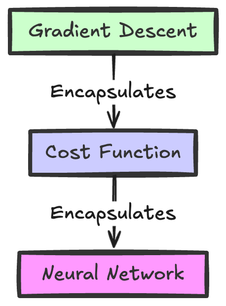
In this post, we’ll explore how the network adjusts its weights and biases to “learn” using a technique called Gradient Descent. (No, this isn’t about hiking uphill, though sometimes it can feel that way!)
How Neural Networks Learn: Gradient Descent
Training a neural network involves feeding it training data—examples of handwritten digits and their correct labels—and adjusting the network’s weights and biases based on its performance. But how exactly does the network make these adjustments?
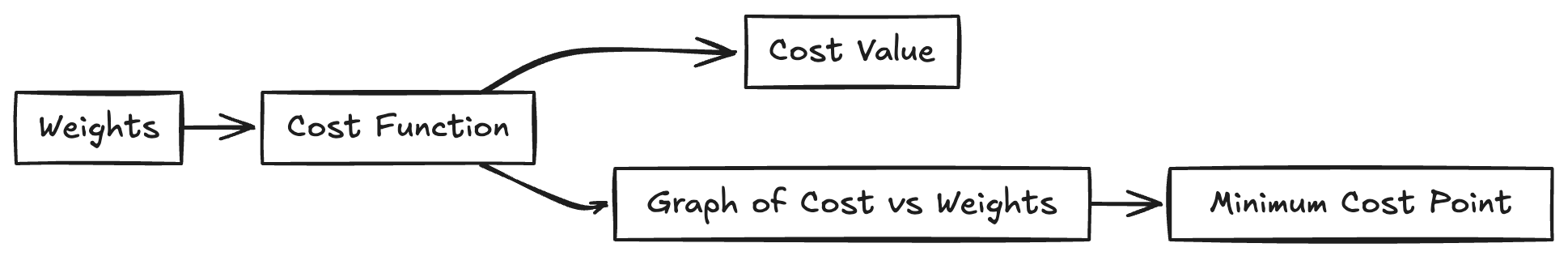
The Role of the Cost Function
To measure how well the network is performing, we use a cost function (or loss function). The cost function computes the difference between the predicted output of the network and the actual correct label for the input. The goal is to minimize this cost over time, meaning we want the network to get better at predicting the correct label. In simpler terms, we’re trying to teach the network to not be so bad at guessing!
Introducing Gradient Descent
Gradient Descent is an optimization algorithm used to minimize the cost function. It works by gradually adjusting the weights and biases in the network, guiding it toward lower and lower cost values. Think of it like this: the network starts off wildly guessing, and each time it guesses wrong, we gently nudge it toward the right answer.
Let’s break it down step by step (pun intended):
Starting Simple: One Parameter, One Slope
Imagine the network has a single weight ( $w$ ), and we plot the cost function based on different values of ( $w$ ). The graph will be a curve showing how the cost changes as ( $w$ ) changes. The point on the curve with the lowest cost is what we want to find—this would be the optimal value of ( $w$ ).
- Pick a Random Starting Point: Start with a random value for ( $w$ ). Let’s be honest, the first guess will be wrong. The network is like a toddler just learning to walk!
- Compute the Slope (Derivative): Find the slope of the cost function at that point. The slope tells us the direction to move:
- If the slope is positive, we need to decrease ( $w$ ).
- If the slope is negative, we need to increase ( $w$ ).
- Adjust ( $w$ ): We adjust ( $w$ ) by a small amount (called the step size or learning rate) in the direction that reduces the cost.
- Repeat: We keep doing this until the slope is very small, meaning we’ve reached a point where further adjustments won’t significantly reduce the cost. This point is called a local minimum. (Yes, the network finally learned to stay standing!)
Expanding to Multiple Parameters: Enter the Gradient
The example above works well when we have just one parameter to adjust. However, neural networks typically have thousands of parameters (weights and biases). In our handwritten digit recognition example, we have 13,002 parameters!
When we have more than one parameter, the concept of a slope (which works in 2D) no longer applies. Instead, we use something called the gradient, which generalizes the idea of a slope to higher dimensions.
Why Switch from Slope to Gradient?
- For one parameter, the slope tells us the direction to move in to minimize the cost.
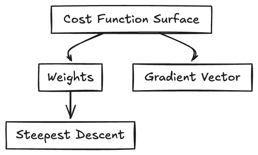
- For multiple parameters, we need to know the direction in a multidimensional space. This is where the gradient comes in. The gradient is a vector that points in the direction of the steepest ascent of the cost function. To minimize the cost, we move in the opposite direction of the gradient (steepest descent).
Gradient Descent in Action
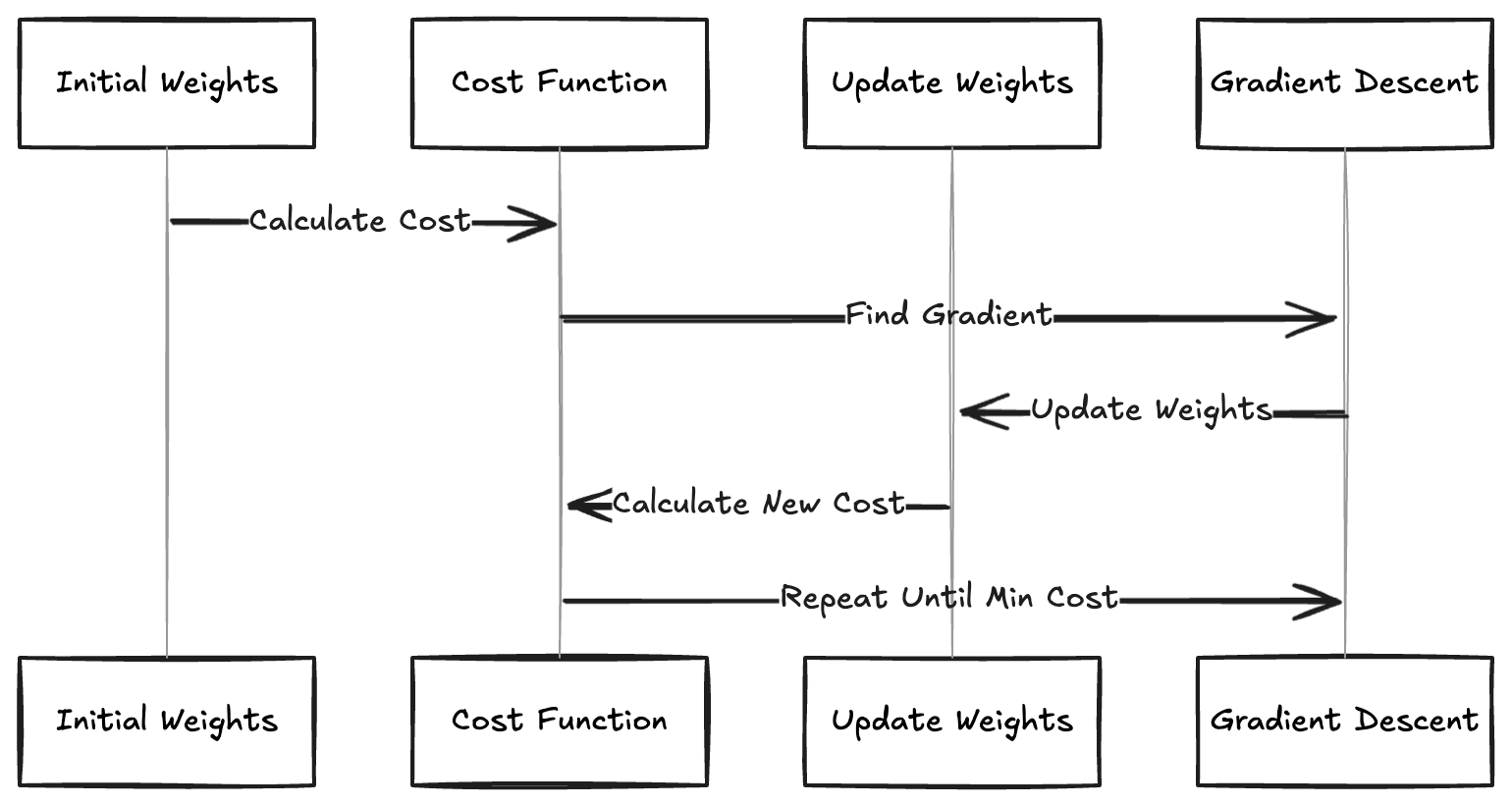
- Start with Random Weights and Biases: Just like in the single-parameter case, we begin by randomly initializing the weights and biases. This is the neural network’s equivalent of going, “Uhhh, let’s try this!”
- Compute the Cost: For each input (a handwritten digit), pass it through the network and calculate the cost using the current weights and biases.
- Find the Gradient: Instead of calculating a single slope, we calculate the gradient of the cost function with respect to each parameter (all 13,002 of them!). You can imagine our weight parameters as ( $w_{1,1}, w_{1,2}, w_{1,3}, \ldots, w_{1,784}$ ) for just the first neuron!
- Update Weights and Biases: Adjust the weights and biases by taking a small step in the negative direction of the gradient. This step ensures we move toward lower cost values.
- Repeat: Continue this process until the gradient becomes very small, indicating that the network has reached a minimum in the cost function (ideally a global minimum, but often we settle for a local minimum).
Gradient Descent Math: A Quick Look
In more mathematical terms, if ( $w ) is a vector of all weights and biases, we update it as follows:
( $w_{new} = w_{old} - \eta \nabla C(w_{old})$ )
Where:
- ( $\eta$ ) is the learning rate (step size).
- ( $\nabla C(\mathbf{w})$ ) is the gradient of the cost function with respect to the weights.
This formula ensures that the weights are updated in the direction that reduces the cost.
Conclusion: Learning Through Gradual Improvement
Gradient Descent is the core mechanism that enables neural networks to “learn.” By iteratively adjusting the weights and biases in response to the cost function, the network gradually improves its predictions. While this process may seem complex, it’s just a series of small, calculated steps toward minimizing error (like training a puppy with treats!).
Share This Post
If you found this post helpful or entertaining, please share it with your friends!
Share on Twitter
Share on Facebook
Share on LinkedIn
Share on Reddit