Understanding Neural Networks: Weights, Biases, and Activations
From Pixels to Predictions: Understanding Neural Networks by Recognizing Handwritten Digits
In our journey through Large Language Models (LLMs), we’ve already taken a detour to explore tokenization (because understanding how data is chopped up and processed is essential). Now, we’re making another (but necessary) detour into neural networks, which form the foundation of everything from image recognition to, yes, LLMs like Transformers.
Before we jump into the famous Attention is All You Need paper (where Transformers show off their power), we need to understand how neural networks process information. To make this fun and easy, we’ll focus on the classic use case of recognizing handwritten digits.
What’s a Neural Network Anyway?
At its core, a neural network is a series of layers made up of neurons (math-based ones, not brain-based ones!). Each neuron is responsible for processing a piece of the input data and passing it through layers of computation until the network arrives at an output — like recognizing a handwritten “7”.
But neural networks aren’t limited to digit recognition. They power everything from image recognition (hello, face filters) to speech recognition (looking at you, Siri) and language models (like the Transformers we’ll eventually get to).
Types of Neural Networks
- Convolutional Neural Networks (CNN): These are great for images. CNNs are used in things like facial recognition, where the network needs to detect patterns and features like eyes, nose, or ears.
- Long Short Term Memory (LSTM): Perfect for sequential data, like speech or time series. Think of them as neural networks with memory, which helps them understand the context in a sequence of words or sounds.
- Multilayer Perceptron (MLP): These are your “basic” neural networks and great for simpler tasks, like recognizing digits. This is where we’ll start.
The Handwritten Digit Recognition Example
Imagine you have a picture of a digit. How can a machine look at it and decide whether it’s a “2” or a “7”? This is where neural networks come into play. Let’s break it down step by step, layer by layer.
Step 1: The Input Layer – Where Pixels Meet Neurons
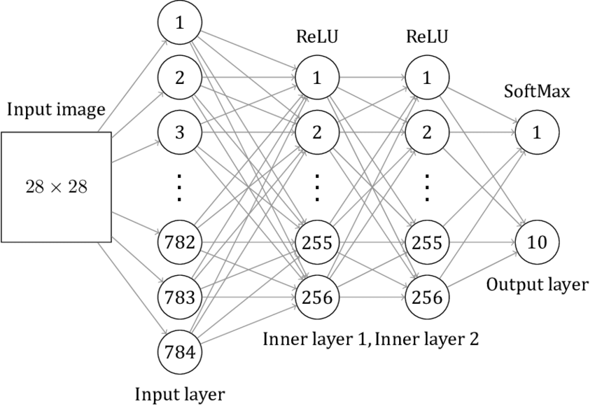
We start with an image of a handwritten digit. Let’s assume this image is a 28x28 grid of pixels (standard for the MNIST dataset used in digit recognition). That’s 784 pixels in total.
Each pixel has a grayscale value between 0 (black) and 1 (white). This grayscale value becomes the activation for each neuron in the input layer. So, the input layer has 784 neurons (one for each pixel).
Example:
- A white pixel (value = 1) might represent the background of the image.
- A black pixel (value = 0) might represent the part of the digit itself.
In essence, the input layer is nothing more than a storage of the pixel values — like a giant grid of grayscale data.
Step 2: The Hidden Layer1 – Extracting Features
After the input layer, we pass the data into hidden layers. These layers perform the heavy lifting: they learn to detect patterns like edges, curves, and corners — the building blocks of digits.
Let’s say our first hidden layer has 16 neurons. Each neuron in this layer will look at a combination of pixels from the input layer and learn to recognize small features, like vertical or horizontal lines (essential to recognizing digits).
Each neuron in the hidden layer is connected to every neuron in the input layer. That’s where the weights come in.
Example: One neuron in the hidden layer might learn to recognize vertical lines. This neuron will be highly “activated” when the input pixels form a vertical stroke (like in the digit “1” or “7”).
Step 3: The Hidden Layer2 – Building Complex Patterns
The next hidden layer might also have 16 neurons. Now the network combines the simpler patterns (like edges and curves) it found in the previous layer to form more complete shapes—like half-circles or straight lines.
This layer helps put the small features together to form a larger picture of what the digit might be.
Step 4: The Output Layer – The Final Guess
After passing through a few hidden layers, we arrive at the output layer. This layer has 10 neurons, one for each digit (0-9). The network will compute which of these neurons has the highest activation value — essentially, which number the network thinks it’s looking at.
Example: If the network’s output neuron for “7” has the highest activation value, it predicts the input image is the number 7.
Now, let’s get to the math of how the network learns to make these predictions.
The Math Behind Neural Networks: Weights, Biases, and Activations
To understand how information is transmitted and how learning happens in a neural network, let’s break down the mathematics behind the process step by step, using the example of the handwritten digit recognition network.
The Key Ingredients
- Input Values (Activations): The values passed from neurons in one layer to the next.
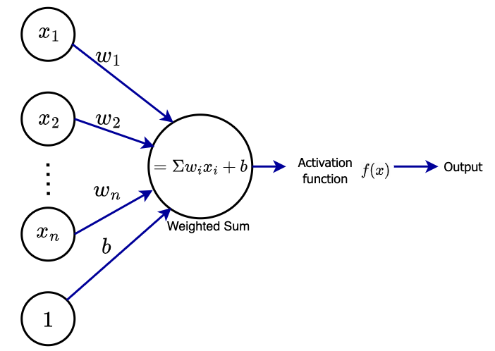
- Weights: Numbers that adjust the importance of each input when passed to the next layer.
- Biases: Extra numbers added to the result to ensure the neuron can activate even if the weighted inputs are small.
- Activation Function: A function (e.g., sigmoid) applied to the result to ensure the output is within a specific range (e.g., between 0 and 1).
Step-by-Step Math
1. Neurons in the Input Layer
- For simplicity, assume the input is a 28x28 grayscale image (784 pixels), where each pixel value is between 0 and 1.
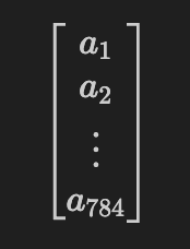
- These pixel values are called activations in the input layer and are denoted by ( $a_1, a_2, \ldots, a_{784}$ ).
2. Weights: Connecting Neurons Between Layers
- Every neuron in the hidden layer receives input from every neuron in the previous layer (the input layer in this case). The connection between each input neuron and a hidden layer neuron is assigned a weight.
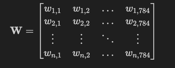
- If the first neuron in the hidden layer is connected to every neuron in the input layer, then the weights associated with this neuron can be represented as ( $w_{1,1}, w_{1,2}, w_{1,3}, \ldots, w_{1,784}$ ).
- Here, ( $w_{1,1}$ ) represents the weight connecting input neuron 1 to the first neuron in the hidden layer, ( $w_{1,2}$ ) for input neuron 2, and so on.
- For neuron ( $j$ ) in the hidden layer, the input is a weighted sum of all inputs:
$z_j = w_{j,1} a_1 + w_{j,2} a_2 + \ldots + w_{j,784} a_{784}$
This is a dot product of the input activations and the weights connecting to that neuron.
3. Bias: Shifting the Weighted Sum
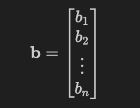
- After calculating the weighted sum for a neuron, a bias is added to this value:
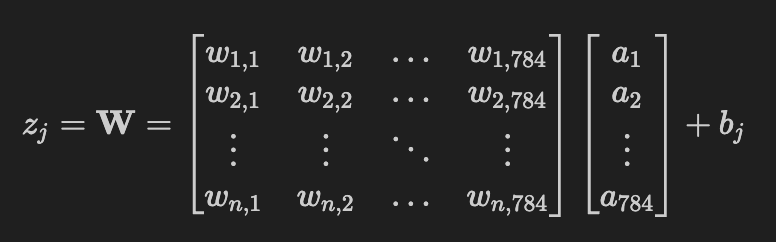
$z_j = w_{j,1} a_1 + w_{j,2} a_2 + \ldots + w_{j,784} a_{784} + b_j$
The bias, ( $b_j$ ), is a number that helps adjust the output of the neuron independently of the inputs.
If we were to represent the above equation as a matrix multiplication:
Weight Vector: Represent the weights as a column vector ($\mathbf{w}_j$) for neuron ($j$):
Activation Vector: Represent the activations as a column vector ($\mathbf{a}$):
Bias Matrix:
Weighted Sum Calculation:
4. Activation Function: Making the Neuron “Fire”
- Once the weighted sum + bias is computed, the result is passed through an activation function to introduce non-linearity into the model.
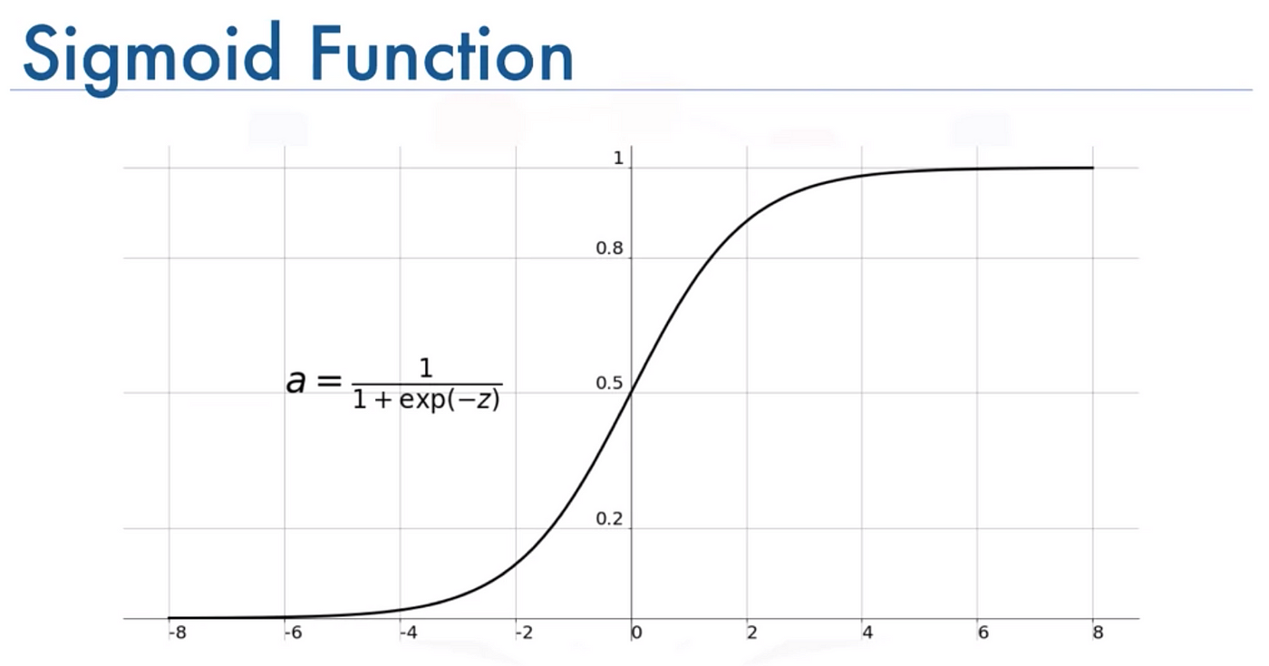
- A commonly used activation function is the sigmoid function:
$\sigma(z) = \frac{1}{1 + e^{-z}}$
The sigmoid squashes the value ( $z$ ) into a range between 0 and 1, making it easier to interpret as a probability.
- So, for neuron ( $j$ ) in the hidden layer, the final output (called the activation for the next layer) is:
$a_j = \sigma(z_j) = \frac{1}{1 + e^{-(w_{j,1} a_1 + w_{j,2} a_2 + \ldots + w_{j,784} a_{784} + b_j)}}$
This value, ( $a_j$ ), is passed to the next layer as an input.
5. Moving to the Next Layer: Repeating the Process
- In the next layer (another hidden layer or the output layer), the process is repeated:
- Take the activations from the previous layer as inputs.
- Multiply them by weights specific to the connections between the current and next layers.
- Add biases.
- Apply the activation function to get the activations for the next layer.
- This process continues until the final output layer.
6. Output Layer: Making the Prediction
- In the output layer, let’s say we have 10 neurons (representing digits 0-9). The output for each neuron is calculated similarly:
$z_k = w_{k,1} a_1 + w_{k,2} a_2 + \ldots + w_{k,n} a_n + b_k$
- This result is passed through a softmax function, which converts the outputs into probabilities that sum to 1:
$\text{softmax}(z_k) = \frac{e^{z_k}}{\sum_{i=1}^{10} e^{z_i}}$
- The neuron with the highest probability is chosen as the network’s prediction of the digit.
A Complete Example
Let’s walk through a simplified example with just a few neurons:
Input Layer (3 pixels for simplicity)
- Assume we have three input pixels with activations ( $a_1 = 0.8$ ), ( $a_2 = 0.4$ ), ( $a_3 = 0.6$ ).
Hidden Layer (2 neurons)
- For the first neuron in the hidden layer, the weights are ( $w_{1,1} = 0.5$ ), ( $w_{1,2} = 0.3$ ), ( $w_{1,3} = -0.2$ ), and the bias is ( $b_1 = 0.1$ ).
The weighted sum:
$z_1 = (0.5 \times 0.8) + (0.3 \times 0.4) + (-0.2 \times 0.6) + 0.1 = 0.4 + 0.12 - 0.12 + 0.1 = 0.5$
- Applying the sigmoid activation:
$a_1 = \sigma(0.5) = \frac{1}{1 + e^{-0.5}} \approx 0.622$
- For the second neuron in the hidden layer, let’s assume the weights are ( $w_{2,1} = -0.3$ ), ( $w_{2,2} = 0.7$ ), ( $w_{2,3} = 0.4$ ), and the bias is ( $b_2 = -0.2$ ).
The weighted sum:
$z_2 = (-0.3 \times 0.8) + (0.7 \times 0.4) + (0.4 \times 0.6) - 0.2 = -0.24 + 0.28 + 0.24 - 0.2 = 0.08$
- Applying the sigmoid activation:
$a_2 = \sigma(0.08) = \frac{1}{1 + e^{-0.08}} \approx 0.52$
Output Layer (2 neurons for a simple binary classification)
- Now, these activations ( $a_1 \approx 0.622$ ) and ( $a_2 \approx 0.52$ ) are passed to the output layer.
- Let’s assume the output neuron weights and biases are such that the final outputs get processed, and through the softmax function, the network predicts either a ‘0’ or ‘1’.
How Does the Network Learn? (aka “Training Time”)
Now that we’ve understood how neurons compute their outputs, let’s talk about learning. Neural networks learn through a process called backpropagation, which adjusts the weights and biases to minimize errors.
Loss Function (aka “How Wrong Were We?”)
To know how well the network performed, we compute the loss, which tells us how far off the network’s prediction was from the actual answer. For digit recognition, we often use a loss function like cross-entropy loss.
Backpropagation (aka “Let’s Fix Those Weights”)
Once we have the loss, the network uses an algorithm called backpropagation to adjust the weights and biases. It goes layer by layer, tweaking the weights to minimize the loss.
In essence, the network tries to get better at predicting digits by reducing its mistakes, adjusting weights and biases until it gets the right answer consistently.
No need to panic! We’ll dive into these concepts in detail after we tackle Transformers.
Why Do We Care About Neural Networks for LLMs and Transformers?
So, why the detour into neural networks? Because neural networks are the building blocks of transformers — the architecture that powers LLMs. While transformers use a more sophisticated mechanism (attention), they share many concepts with neural networks, including:
- Layer-based processing (data passes through multiple layers).
- Weights and activations (used to adjust how data is processed).
- Learning via training data.
Understanding neural networks gives us a solid foundation to dive into attention mechanisms and understand why transformers are so powerful in tasks like language translation and text generation.
Wrapping Up: From Digits to Deep Learning
To summarize:
- Neural networks process data layer by layer, using weights and biases to compute results.
- Hidden layers extract features (like edges or curves) that help the network recognize patterns.
- Through training, the network adjusts its weights and biases to make better predictions.
Understanding neural networks is like learning the alphabet before you dive into writing novels — and soon, we’ll be diving into Transformers and how they use the attention mechanism to take neural networks to the next level.
“Feeling a bit lost? Don’t worry! Dive into this GH repository where the code does all the talking. Trust me, it’s way more informative than I this blog!”
Until next time, keep those neurons firing!
Share This Post
If you found this post helpful or entertaining, please share it with your friends!
Share on Twitter
Share on Facebook
Share on LinkedIn
Share on Reddit